Passive Crossover for Bookshelf Speakers
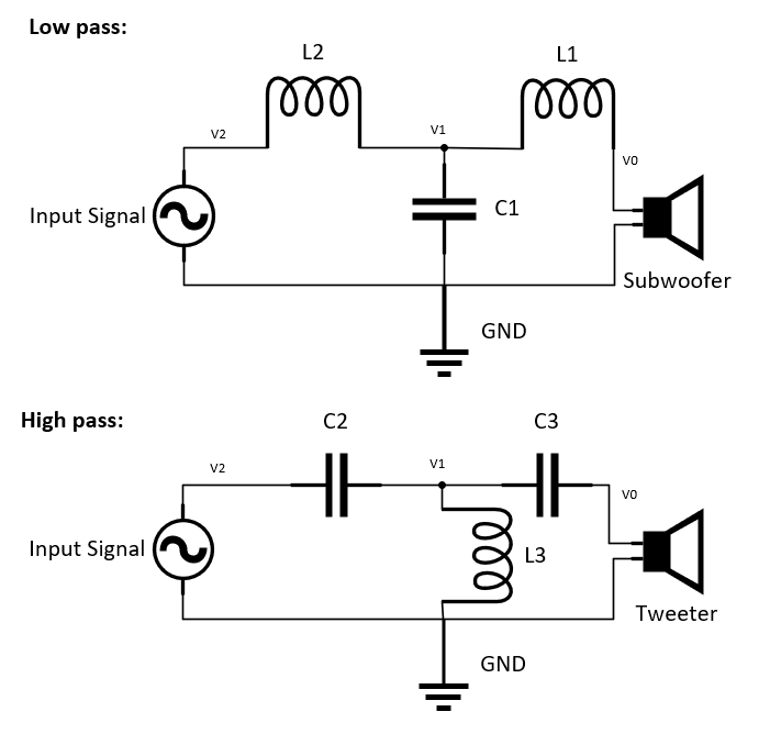
I wanted to create a passive crossover for a two-way speaker system. The job of a two-way crossover is to split up an audio signal such that the woofer is fed the low frequency signal, and the tweeter is fed the high frequency signal. This way, each driver is only operating within the frequency range it can accurately reproduce sound in. If this is done well, the combined frequency response from all the drivers should seamlessly act as if they were one full-range driver.
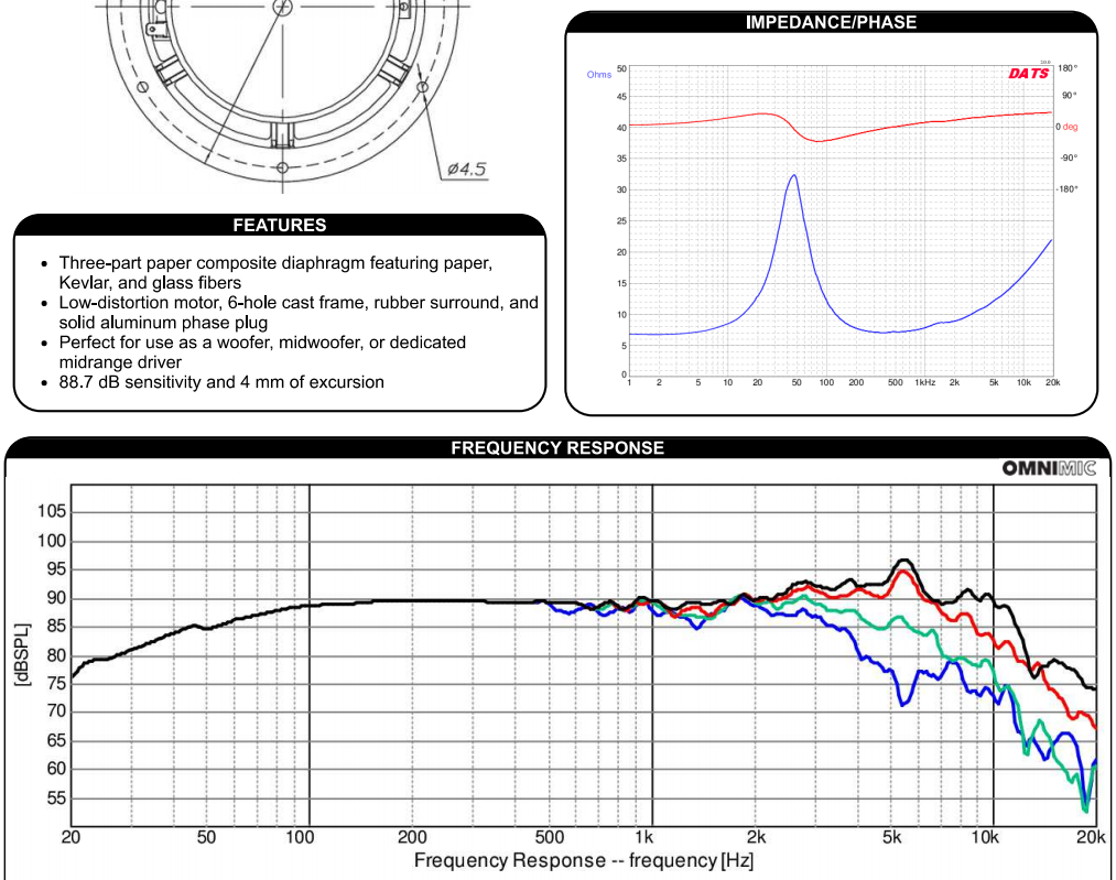
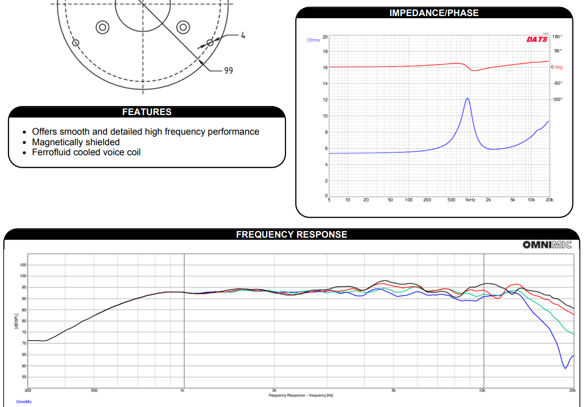
When designing a crossover, there are two main plots to look at in the drivers’ datasheets: the frequency response, and the impedance. The frequency response is important because it dictates how the drivers will sound. The impedance is used in the filter calculations.
My objective for the crossover design was to try and maintain as much audio fidelity as possible while sticking to affordable drivers. The ideal combined response is of course a flat light between 20Hz and 20kHz. I selected a mid-bass driver and tweeter with the flattest frequency response I could find in the price range and form factor I was looking for.
Mid-bass
Tweeter
For this project I used a 3rd order filter which has an 18dB/decade slope after the cutoff frequency.
The speakers’ impedance change with respect to frequency according to the datasheet. However, relative to the inductors and capacitors, they do not change significantly. I am going to explain the analysis by modeling the drives each as an 8ohm resistor, however in my code I used the impedance provided by the datasheet. I am only going to walk through the analysis for the low pass filter, but the analysis for the high pass side is the same.
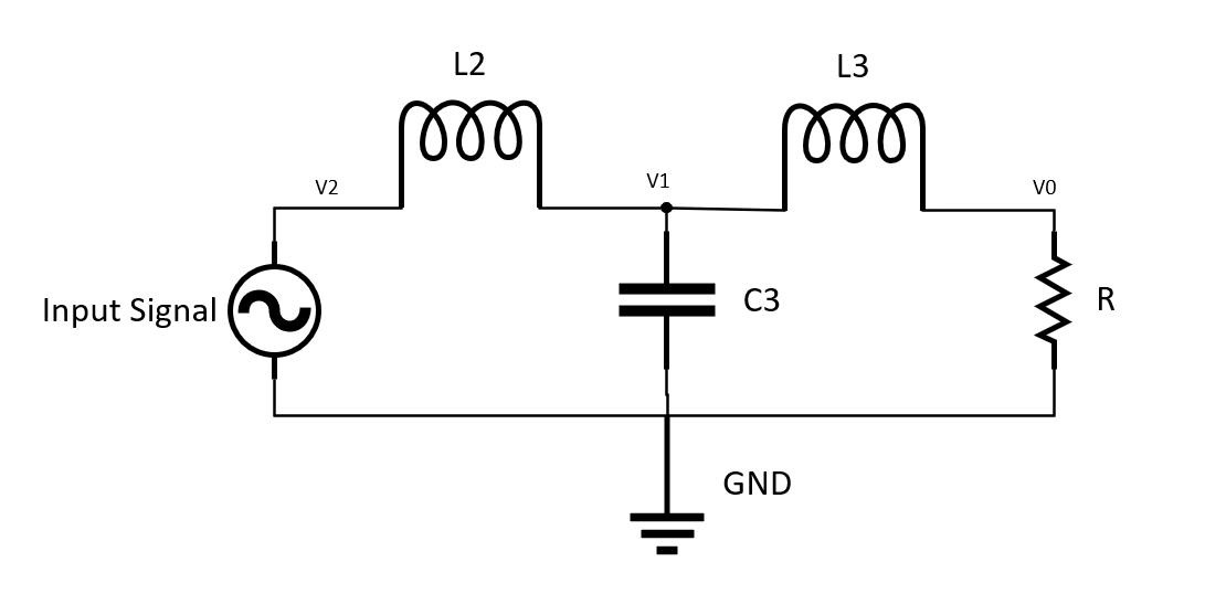
The goal of this analysis is to solve for the gain of the filter as a function of frequency which in this case is \(\frac{V_0}{V_2}\). The first step is to solve for the impedance the inductors and capacitors using equations 1 and 2 respectively.
\(
Z_L = 2\pi fL
\).
Equation 1
Where:
Z = Impedance
\(f\) = Frequency
L = Inductance
\(
Z_C = \frac{1}{2\pi f C}
\).
Equation 2
Where:
Z = Impedance
\(f\) = Frequency
C = Capacitance
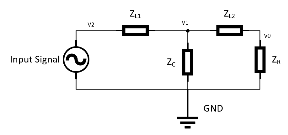
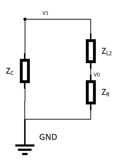
Before we can solve for \(\frac{ V0}{V2}\), we must solve for \(\frac{ V1}{V2}\). First, we will solve for the effective impedance of \(Z_c\), \(Z_{L2}\), and \(Z_R\) which we will call \(Z_3\). This is solved using equation 3.
\(
Z_3 = \frac{1}{1/(Z_C)+1/(Z_R+Z_{L2})}
\).
Equation 3
This circuit then simplifies as shown below.
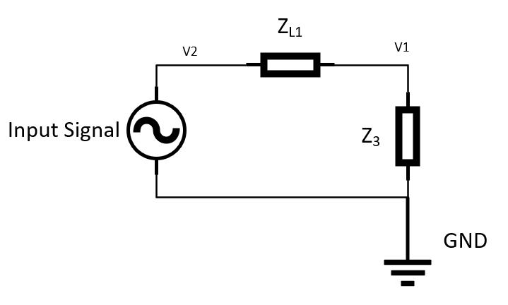
\(\frac{ V1}{V2} = \frac{Z_3}{Z_3+Z_{L1}}\)
Next \(\frac{V0}{V1}\) can be found using another voltage divider.
\(\frac{V0}{V1} = \frac{Z_R}{Z_R+Z_{L2}}\)
Finally we can solve for the gain.
\(G_{low} = \frac{V0}{V1} \frac{V1}{V2} = \frac{V0}{V2}\)
The gain is then applied to the frequency response of the woofer. You can see in the figure below how the high frequency response is attenuated, while the low frequency response remains unchanged. The opposite is true for the tweeter.
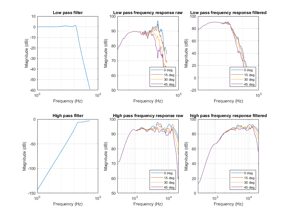
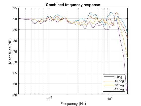
The total frequency response is simply the sum of the filtered tweeter and woofer’s response.
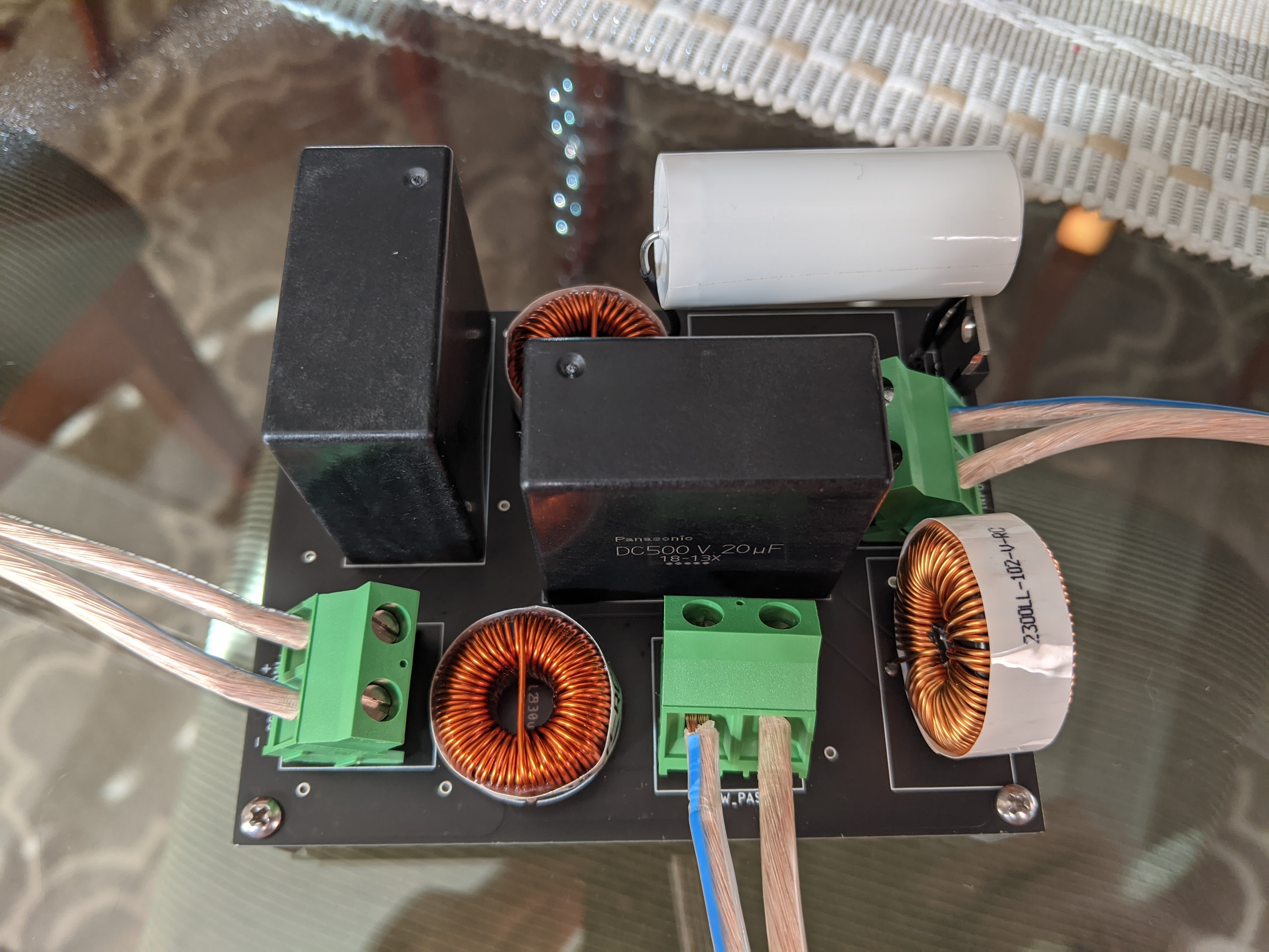
Below is an image of what the crossover looked like after I populated the board.
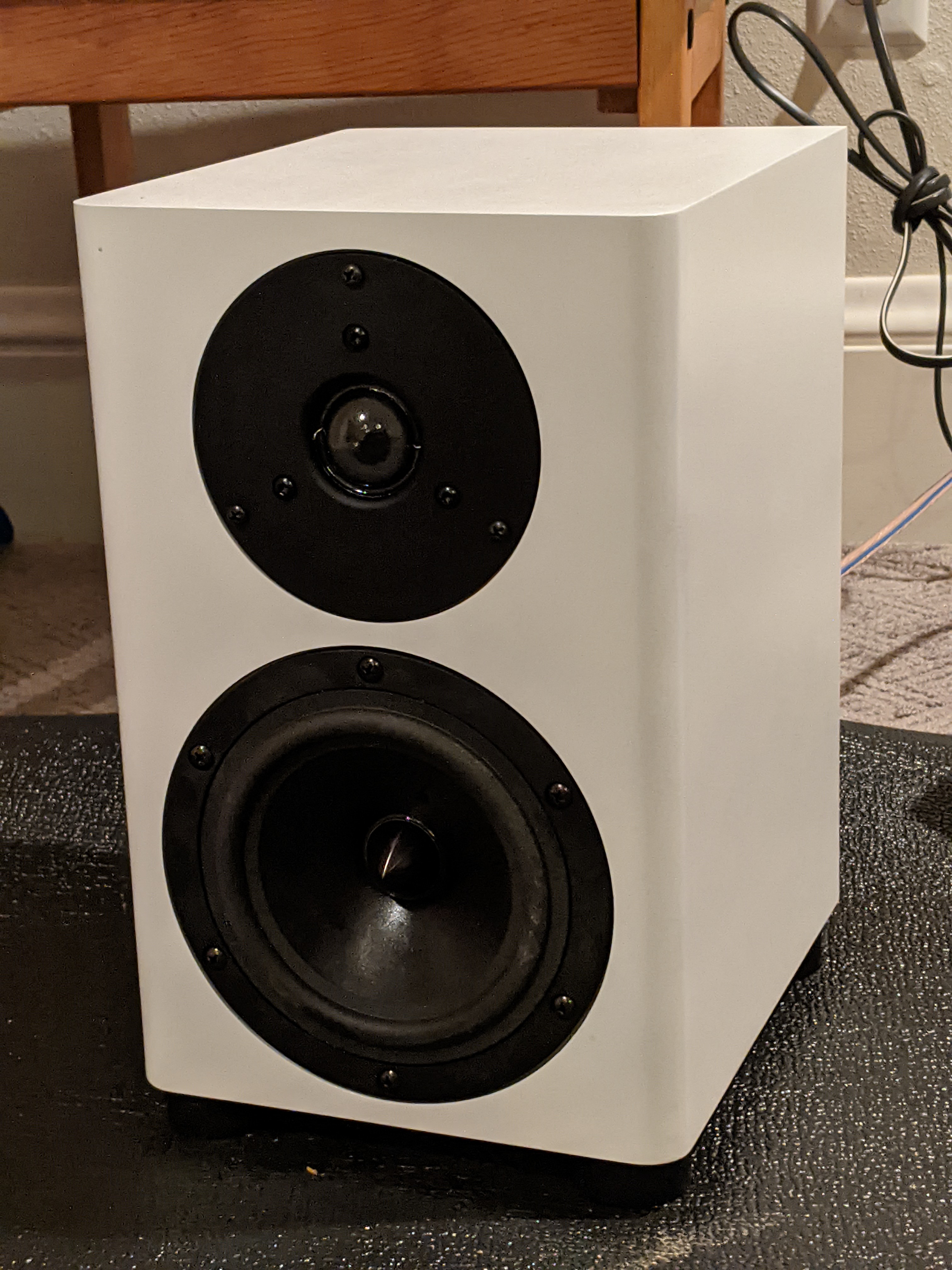
This is what they looked like when they were done! They sound great. This project has motived me to build another pair at some point. I think next time I want to try my hand at a three-way crossover.
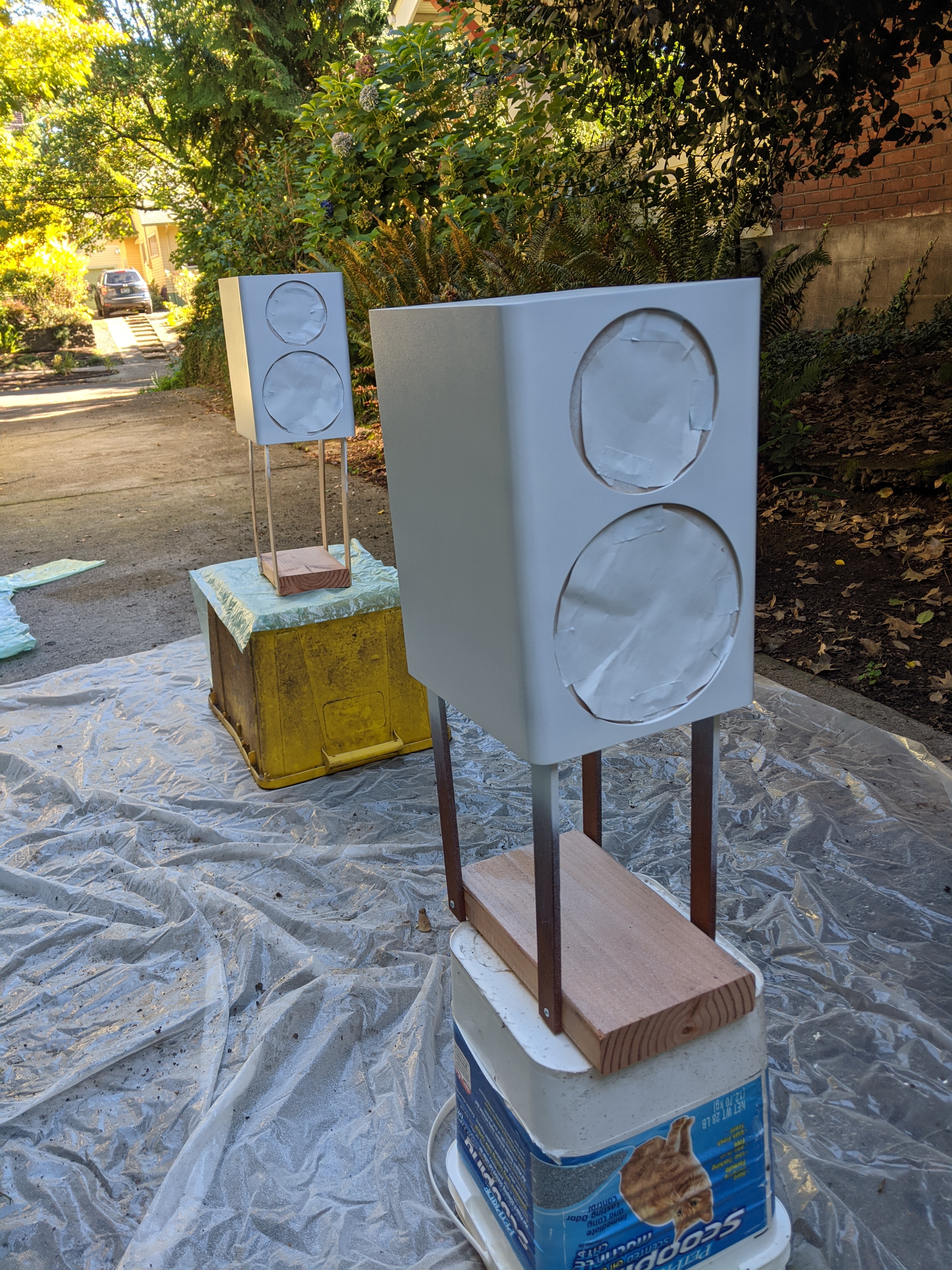
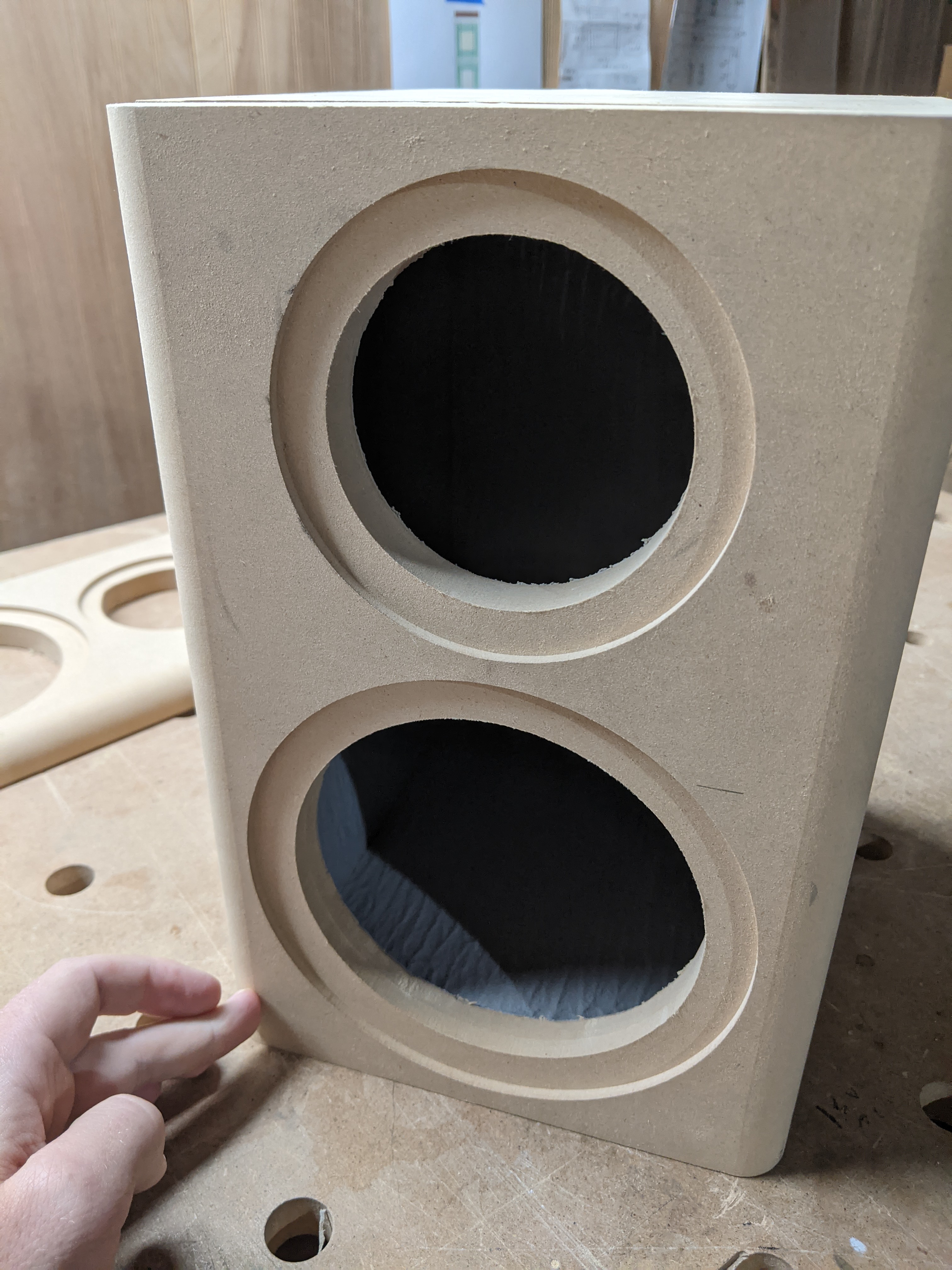
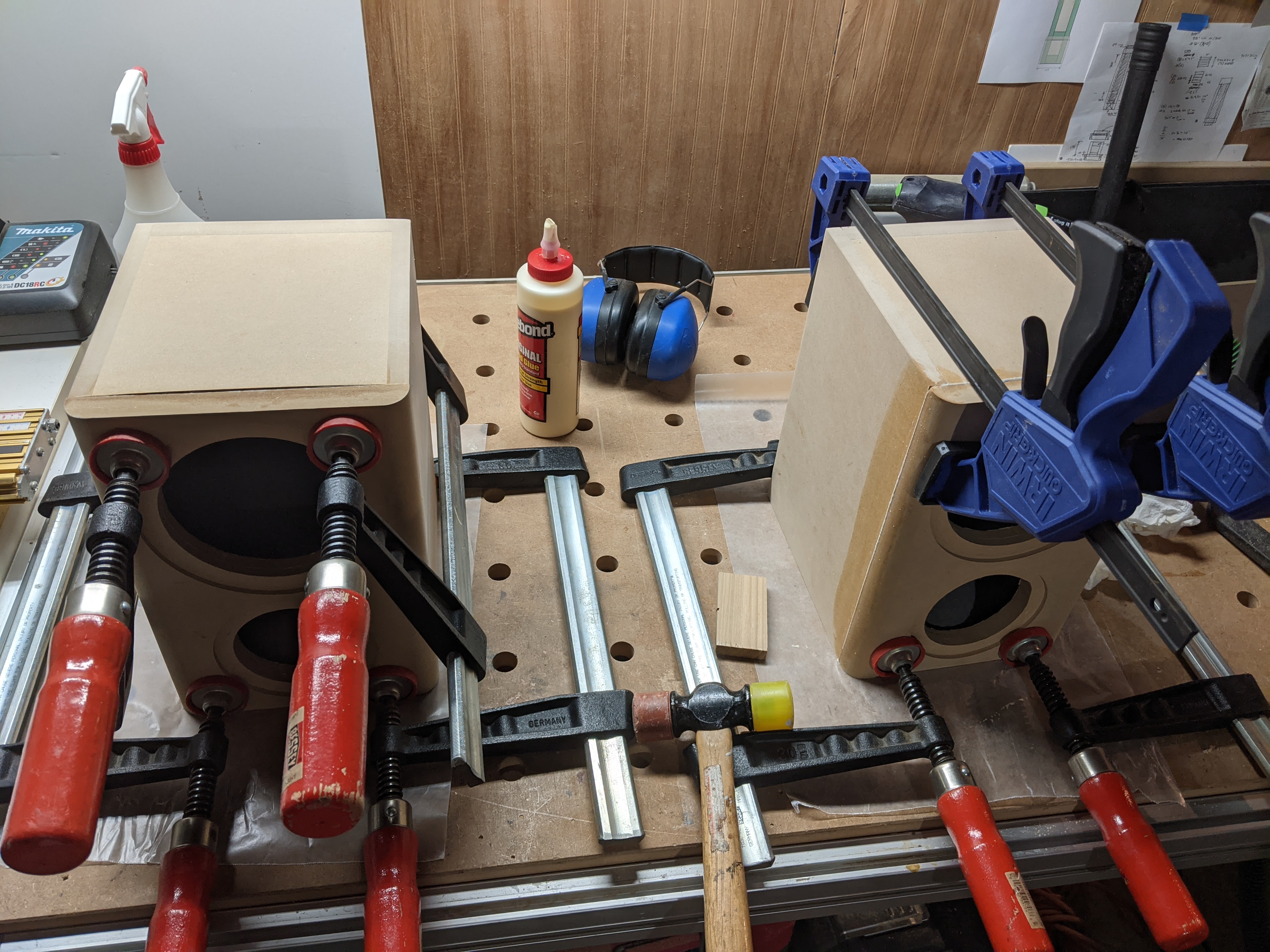
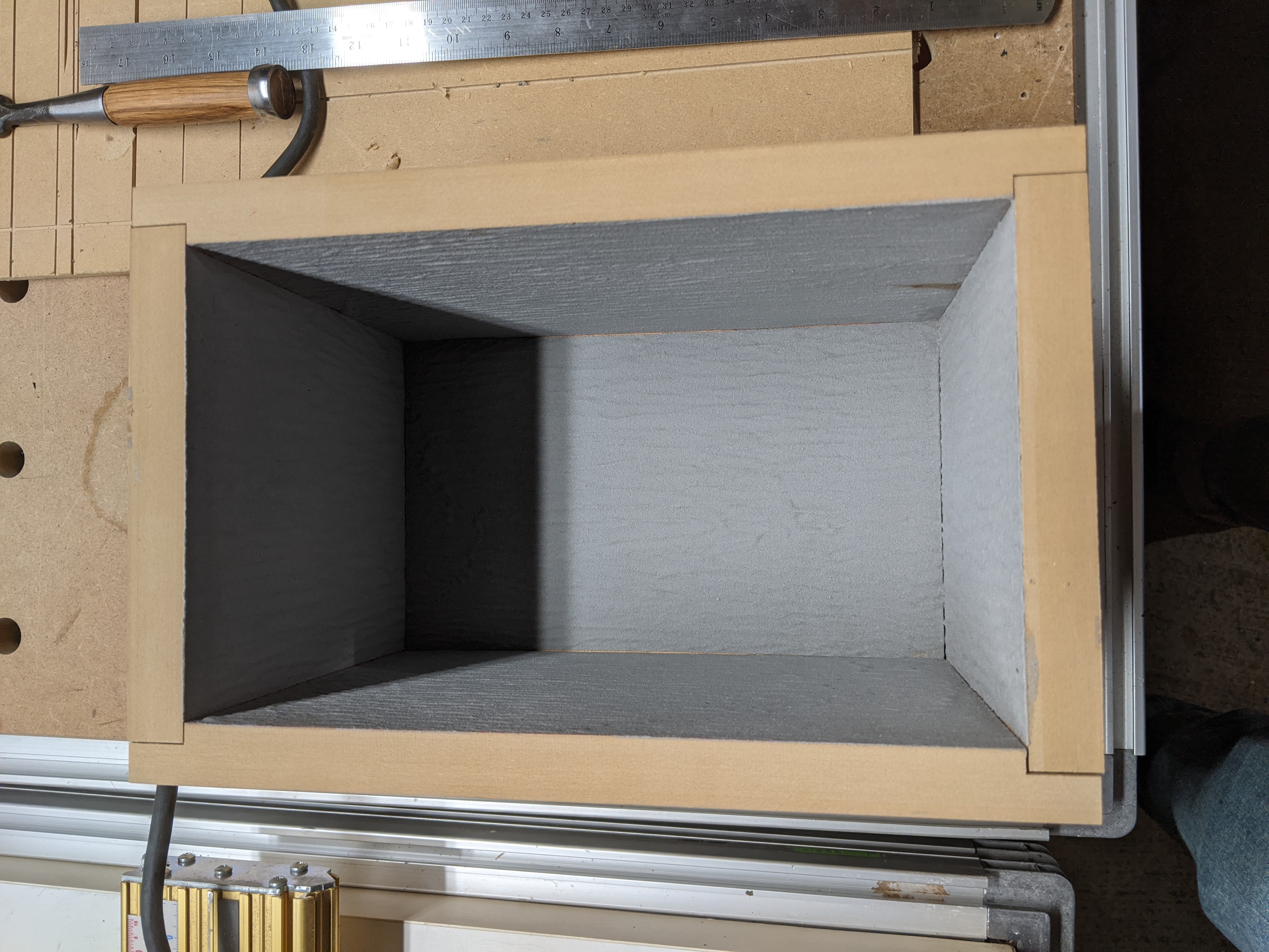
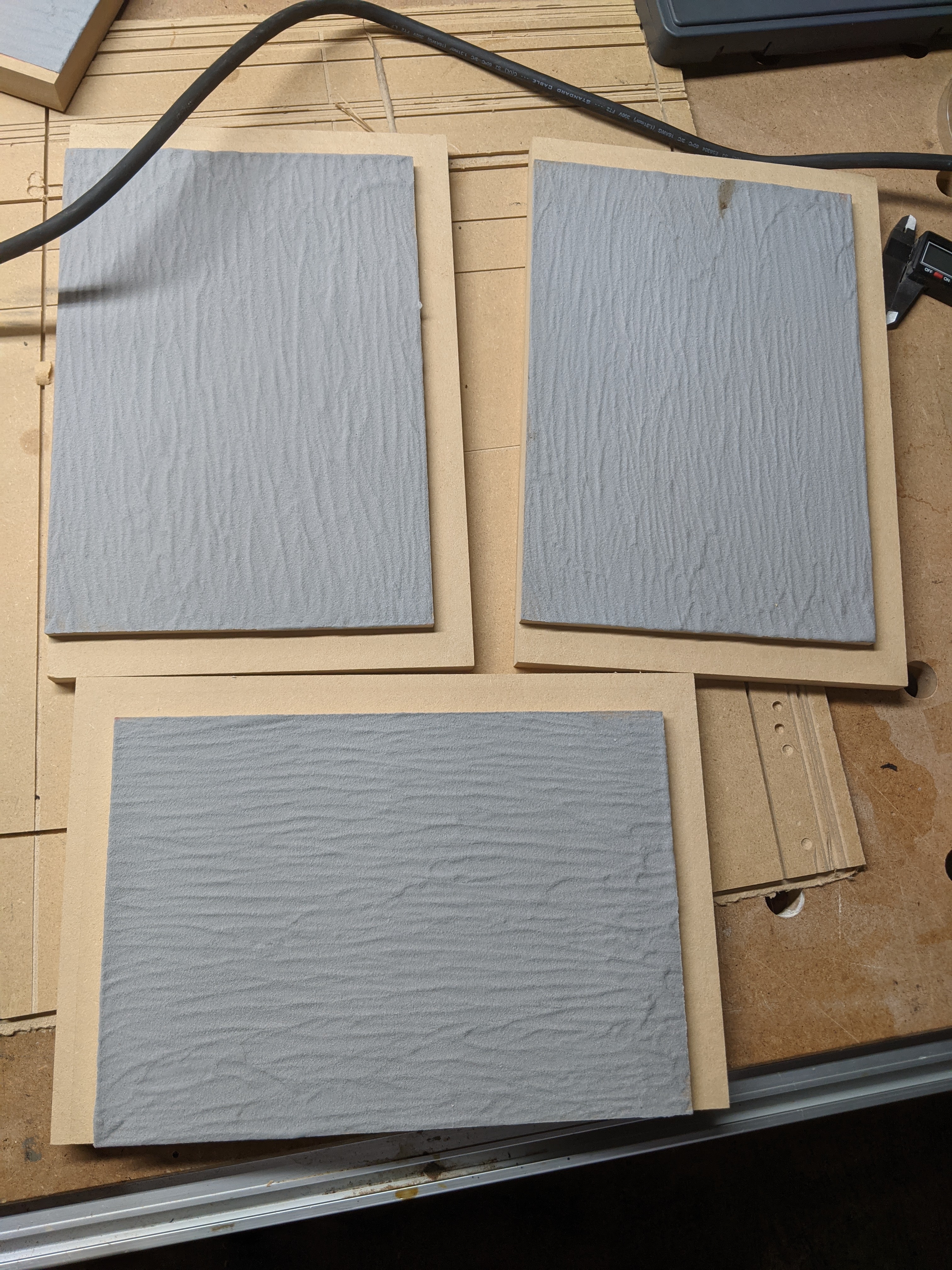
I am going to skip explaining the woodworking process, but here is a gallery of my progress along the way.
You can find my code down below if you are interested.
    clc
    clear
    clf
    close all;

    %% Component Values
    % low pass filter
    C_low = 20*10^-6;%F
    L1_low = 1*10^-3;%H
    L2_low = 0.33*10^-3;%H
    % high pass filter
    C1_high = 5*10^-6;%F
    C2_high = 15*10^-6;%F
    L_high = 0.33*10^-3;%H
    R_high = 5;%ohms

    %% import data
    %Import mid-bass impedance and define independent variable
    mid_data = readtable("C:\Users\coled\Desktop\Speaker Project\8 Ohm design\Mid-8-RS150P.csv");
    f = table2array(mid_data(:,1));
    zm_mid = table2array(mid_data(:,2));
    phi_mid = table2array(mid_data(:,3));
    z_mid = zm_mid.*cosd(phi_mid)+i.*zm_mid.*sind(phi_mid); %Define in rectangular coordinates
    %Import mid-bass frequency response
    mid_data_freq_0 = readtable("C:\Users\coled\Desktop\Speaker Project\8 Ohm design\Mid-8-RS150P-freq-0.csv");
    mid_data_freq_15 = readtable("C:\Users\coled\Desktop\Speaker Project\8 Ohm design\Mid-8-RS150P-freq-15.csv");
    mid_data_freq_30 = readtable("C:\Users\coled\Desktop\Speaker Project\8 Ohm design\Mid-8-RS150P-freq-30.csv");
    mid_data_freq_45 = readtable("C:\Users\coled\Desktop\Speaker Project\8 Ohm design\Mid-8-RS150P-freq-45.csv");
    %Import tweeter impedance and frequency response
    tweet_data = readtable("C:\Users\coled\Desktop\Speaker Project\8 Ohm design\Tweet-8-CD28FS.csv");
    tweet_data_freq_0 = readtable("C:\Users\coled\Desktop\Speaker Project\8 Ohm design\Tweet-8-CD28FS-freq-0.csv");
    tweet_data_freq_15 = readtable("C:\Users\coled\Desktop\Speaker Project\8 Ohm design\Tweet-8-CD28FS-freq-15.csv");
    tweet_data_freq_30 = readtable("C:\Users\coled\Desktop\Speaker Project\8 Ohm design\Tweet-8-CD28FS-freq-30.csv");
    tweet_data_freq_45 = readtable("C:\Users\coled\Desktop\Speaker Project\8 Ohm design\Tweet-8-CD28FS-freq-45.csv");
    zm_tweet = table2array(tweet_data(:,2));
    phi_tweet = table2array(tweet_data(:,3));
    z_tweet = zm_tweet.*cosd(phi_tweet)+i.*zm_tweet.*sind(phi_tweet); %Define in rectangular coordinates

    %% low pass filter
    %calcualte impedance of low pass filter components
    Z_c_low = -i*1./(2*pi*f*C_low);%Ohms
    Z_l1_low = i*2*pi*f*L1_low;%Ohms
    Z_l2_low = i*2*pi*f*L2_low;%Ohms
    Z_1_low = 1./(1./Z_c_low + 1./(Z_l2_low + z_mid));
    %calculate gain of filter breaking the circuit down into two voltage
    %dividers.
    V1_low = mag_of_complex(Z_1_low)./mag_of_complex(Z_1_low + Z_l1_low);
    V0_low = V1_low.*mag_of_complex(z_mid)./mag_of_complex(Z_l2_low + z_mid);
    %create filter bode plot
    subplot(2,3,1)
    semilogx(f,20*log10(V0_low))
    grid on
    xlabel("Frequency (Hz)")
    ylabel("Magnitude (dB)")
    title("Low pass filter")
    %% Mid freq response raw
    %align x axis with other data so all variables agree on frequency
    f_unsynced = table2array(mid_data_freq_0(:,1));
    mid_freq_unsynced_0 = table2array(mid_data_freq_0(:,2));
    mid_freq_unsynced_15 = table2array(mid_data_freq_15(:,2));
    mid_freq_unsynced_30 = table2array(mid_data_freq_30(:,2));
    mid_freq_unsynced_45 = table2array(mid_data_freq_45(:,2));
    for k = 1:length(f)
        mid_freq_0(k) = interp1(f_unsynced,mid_freq_unsynced_0,f(k));
        mid_freq_15(k) = interp1(f_unsynced,mid_freq_unsynced_15,f(k));
        mid_freq_30(k) = interp1(f_unsynced,mid_freq_unsynced_30,f(k));
        mid_freq_45(k) = interp1(f_unsynced,mid_freq_unsynced_45,f(k));
    end
    %convert from dB to linear scale
    mid_freq_0 = 10.^(mid_freq_0/20);
    mid_freq_15 = 10.^(mid_freq_15/20);
    mid_freq_30 = 10.^(mid_freq_30/20);
    mid_freq_45 = 10.^(mid_freq_45/20);
    subplot(2,3,2)
    %create bode plot of unfiltered mid-bass frequency response
    semilogx(f,20*log10(mid_freq_0));
    hold on
    grid on
    semilogx(f,20*log10(mid_freq_15));
    semilogx(f,20*log10(mid_freq_30));
    semilogx(f,20*log10(mid_freq_45));
    xlabel("Frequency (Hz)")
    ylabel("Magnitude (dB)")
    title("Low pass frequency response raw")
    legend("0 deg","15 deg","30 deg","45 deg",'Location','southeast')

    %% Mid freq filtered
    %create bode plot of filtered mid-bass frequency response by applying gain
    subplot(2,3,3)
    semilogx(f,20*log10(V0_low'.*mid_freq_0));
    hold on
    grid on
    semilogx(f,20*log10(V0_low'.*mid_freq_15));
    semilogx(f,20*log10(V0_low'.*mid_freq_30));
    semilogx(f,20*log10(V0_low'.*mid_freq_45));
    xlabel("Frequency (Hz)")
    ylabel("Magnitude (dB)")
    title("Low pass frequency response filtered")
    legend("0 deg","15 deg","30 deg","45 deg",'Location','southeast')

    %% high pass filter
    %calcualte impedance of high pass filter components
    Z_l_high = 2*pi*f*L_high*i;%Ohms
    Z_c1_high = -i*1./(2*pi*f*C1_high);%Ohms
    Z_c2_high = -i*1./(2*pi*f*C2_high);%Ohms
    Z_1_high = 1./(1./Z_l_high + 1./(Z_c2_high + z_tweet));
    %calculate gain of filter breaking the circuit down into two voltage
    %dividers.
    V1_high = mag_of_complex(Z_1_high)./mag_of_complex(Z_1_high + Z_c1_high + R_high);
    V0_high = V1_high.*mag_of_complex(z_tweet)./mag_of_complex(Z_c2_high + z_tweet);
    %create filter bode plot
    subplot(2,3,4)
    semilogx(f,20*log10(V1_high))
    grid on
    xlabel("Frequency (Hz)")
    ylabel("Magnitude (dB)")
    title("High pass filter")
    %% Tweet freq response raw
    subplot(2,3,5)
    %align x axis with other data so all variables agree on frequency
    f_unsynced = table2array(tweet_data_freq_0(:,1));
    tweet_freq_unsynced_0 = table2array(tweet_data_freq_0(:,2));
    tweet_freq_unsynced_15 = table2array(tweet_data_freq_15(:,2));
    tweet_freq_unsynced_30 = table2array(tweet_data_freq_30(:,2));
    tweet_freq_unsynced_45 = table2array(tweet_data_freq_45(:,2));
    for k = 1:length(f)
        tweet_freq_0(k) = interp1(f_unsynced,tweet_freq_unsynced_0,f(k));
        tweet_freq_15(k) = interp1(f_unsynced,tweet_freq_unsynced_15,f(k));
        tweet_freq_30(k) = interp1(f_unsynced,tweet_freq_unsynced_30,f(k));
        tweet_freq_45(k) = interp1(f_unsynced,tweet_freq_unsynced_45,f(k));
    end
    %convert from dB to linear scale
    tweet_freq_0 = 10.^(tweet_freq_0/20);
    tweet_freq_15 = 10.^(tweet_freq_15/20);
    tweet_freq_30 = 10.^(tweet_freq_30/20);
    tweet_freq_45 = 10.^(tweet_freq_45/20);
    %create bode plot of unfiltered tweeter frequency response
    semilogx(f,20*log10(tweet_freq_0));
    hold on
    grid on
    semilogx(f,20*log10(tweet_freq_15));
    semilogx(f,20*log10(tweet_freq_30));
    semilogx(f,20*log10(tweet_freq_45));
    xlabel("Frequency (Hz)")
    ylabel("Magnitude (dB)")
    title("High pass frequency response raw")
    legend("0 deg","15 deg","30 deg","45 deg",'Location','southeast')

    %% tweet freq filtered
    %create bode plot of filtered tweeter frequency response by applying gain
    subplot(2,3,6)
    semilogx(f,20*log10(V0_high'.*tweet_freq_0));
    hold on
    grid on
    semilogx(f,20*log10(V0_high'.*tweet_freq_15));
    semilogx(f,20*log10(V0_high'.*tweet_freq_30));
    semilogx(f,20*log10(V0_high'.*tweet_freq_45));
    xlabel("Frequency (Hz)")
    ylabel("Magnitude (dB)")
    title("high pass frequency response filtered")
    legend("0 deg","15 deg","30 deg","45 deg",'Location','southeast')

    %% Total response
    figure(7)
    %add frequency responses together and convert to dB
    semilogx(f,20*log10(V0_low'.*mid_freq_0 + V0_high'.*tweet_freq_0));
    hold on
    grid on
    semilogx(f,20*log10(V0_low'.*mid_freq_15 + V0_high'.*tweet_freq_15));
    semilogx(f,20*log10(V0_low'.*mid_freq_30 + V0_high'.*tweet_freq_30));
    semilogx(f,20*log10(V0_low'.*mid_freq_45 + V0_high'.*tweet_freq_45));
    xlabel("Frequency (Hz)")
    ylabel("Magnitude (dB)")
    title("Combined frequency response")
    legend("0 deg","15 deg","30 deg","45 deg",'Location','southeast')